How to set up local automatic testing
Test driven development
Test driven development is simple:
- RED: Think about the scientific result that should be achieved and prepare corresponding tests (input data for your testing application).
- A test for an interpolation method is a comparison between interpolated and exact values.
- A test for a polygon / halfspace intersection algorithm is a set of 50 tests that check for valid outputs of epsilon-perturbed data.
- GREEN: Program a testing application and make the test run that reports a quantifiable error.
- Quantifiable: timing of an algorithm, L_1, L_inf error, etc.
- The test application will define the interface for the algorithm: be it a set of functions/routines (fortran), or a set of member functions (C++). Example: compute the signed distance field (calcSignedDistance), intersect the surface mesh with the volume mesh (intersectMeshes), set volume fraction values (calcVolFraction).
- REFACTOR: Improve your source code.
- Improve the accuracy of the algorithm, improve the speed of execution.
- Improve the interface of the algorithm: separate large functions into smaller ones, reorganize private data in the class (what can be passed as an argument and what should be kept as an internal reference), etc.
Automating tests
A single test usually only helps in getting the first implementation right. A scientific result involves parameterization of the test with either a randomized or somehow structured parameter space.
-
Step 1: Modify either the RED or the GREEN step to create the input data parameterization. If you modify the RED step, you will modify the input data in a scripted way (suggestion: python or bash , or pyFoam for OpenFOAM), and generate many simulation cases. Each simulation case (input file) corresponds to a vector in your parameter space. If you modify the GREEN step, the test application will be modified to change the initial (+boundary) conditions (input data).
-
Step 2: Make the testing application write a CSV file with columns named after the errors / timings you want to test:
Nt,Nb,Ev,Ti,Te,Nx,Ni,Nk
2268,64,9.88206304474011e-09,0.317855331,0.040374638,2429,10,54
2268,64,4.9410381488119e-09,0.317855331,0.033364076,2384,8,56
2268,64,4.94119534273804e-09,0.317855331,0.032788723,2383,8,56
2268,64,4.94102415965688e-09,0.317855331,0.034525081,2424,10,54
…There will be one such file, with a table inside, per test case. The rows are evolving time steps, convergence iterations, random input data perturbations, etc. The file can also only have two lines: named columns and a single data line. This is a result of a single test case in a parameter variation study.
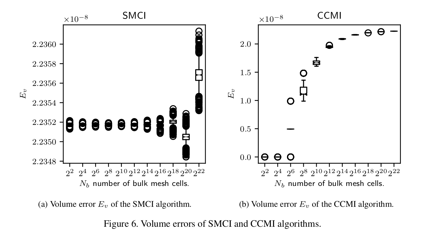
At this point a set of tables is generated, where each table corresponds to a vector in the parameter space. These tables are not reported in a publication usually, instead, box plots are reported for distributions, in addition with diagrams and tables that show the behavior of different error norms. In order to do this, the tables generated by the parameter study need to be agglomerated.
-
Step 3: Agglomerate the CSV files to report the output of the parameterization.
Use pandas , the Python library for data science:
- It can address the columns using their names, there is no need to remember which column is where.
- It can plot box-plots and do complex data analysis of such data frames using single-line commands.
- It exports the tables to LaTeX , stores them into files, that can be automatically included into a report.
Depending on how your simulation software works, the tables are going to be generated and stored either in the same folder, or in different folders.
If they are stored in the same folder, they should be named differently, so that the parameter vector can be determined from their name. For example:
3Ddeformation-HPCToolkit-resolution-00128-process-000-AdvectionWait-scaling.csvhas a naming conventiontestCase-profilinSoftware-meshResolution-N-mpiProcess-M-description.csvand a content:P,Tp,Lin
4.0,1154.66,1154.66
8.0,973.05,577.33
16.0,915.46,288.665
32.0,648.7,144.3325
64.0,441.38,72.16625The naming of the file and its content are defined in the GREEN step, in your testing application. It opens the file, and dumps the measurement data together with the column name line into a file.
OpenFOAM parameter studies are usually configured such that a new simulation folder is created per parameter study vector. This prevents errors that happen when different simulation processes try to read the same files from the disk, if one tries to execute all of them at the same time on a high performance cluster. For OpenFOAM, there is a great tool called pyFoam that already provides an application for generating a parameter study, preparing all the cases and storing the variation vectors into a SQLite database or a text file. The application to be used for that is called
pyFoamRunParameterVariation.py.In the case when the parameter simulations are stored in different folders, either the names of the folders will identify the parameter space vector, or there will be a file (e.g. input file of your simulation program), that identifies the parameter vector and relates it to the CSV file that holds the data.
The mapping between the data file (in CSV or any other format) generated for the parameter study, and the parameter vector is a necessary requirement for analyzing the behavior of the program as a distribution of parameter vector values. Example: how is L_1 error scaling with increased mesh resolution (convergence study) across all CFL numbers and mesh types? The distribution L_1(cell shape, mesh resolution, CFL) requires all tables with L_1 in the column line to be inserted into a larger, multidimensional table that allows multidimensional indexing.
Alternatively, the data is not stored into a CSV file by the post-processesing application, instead HDF5 format is used, that allows storing metadata together with the data. The metadata can then contain, among other things, the components of the parameter vector. Still, files should be named differently obviously, in case a program does not create separate directories for each parameter vector, so that the files will not be overwritten.
In all cases, once the data file is mapped to the parameter vector, all such files should be read by an application (strong suggestion: use python and pandas) and agglomerated together. The code snipppet below shows how this is done for a case where the files are stored in different directories:
def agglomerate_data(intersectionType):
	"""Agglomerates all the data frames from a parameter study into a single dataframe."""
	dirs = intersection_dirs(intersectionType)
	dirs.sort()

	# Assumes the same number of iterations in the experiment: the index of every
	# CSV file should therefore have the same length.
	csvFileName = os.path.join(os.curdir, dirs[0], intersectionType + '.csv')
	csvDf = pd.read_csv(csvFileName)
	iterationList = list(csvDf.index)
	clmns = csvDf.columns


	# Data frames picked up from CSV files stored in simulation directories.
	dfs = []
	# A list of mesh resolution numbers N, where N^2 is the number of base mesh cells in 2D
	# and N^3 is the number of base mesh cells in 3D. Used for indexing specific cases. Nb
	# stores the total number of cells used anyway.
	resolutionList = []
	for directory in dirs:
		csvFileName = os.path.join(os.curdir, directory, intersectionType + '.csv')
		csvDf = pd.read_csv(csvFileName)
		meshResolutionN = int(sqrt(csvDf["Nb"].iloc[0]))
		resolutionList.append(meshResolutionN)
		dfs.append(csvDf)

	# Store all data in a df with a multidimensional index
	mIndex = pd.MultiIndex.from_product([resolutionList, iterationList],
										names=['N', 'iteration'])

	agglDf = pd.concat(dfs)
	agglDf.index = mIndex

	return agglDf
Notice ‘pd.MultiIndex’: learn about pandas MultiIndex, it makes it possible to have tables with multi-dimensional indexing, that perfectly fits to parameter studies with a cartesian product of parameter vectors. In this case, there are two parameters: resolution of the mesh and the number of iterations used for the randomly perturbed input.
Notice ‘pd.concat(dfs)’: adding data frames (CSV tables) to each other is trivial. Once the multiindex has been set up, a multidimensional table can be simply created by concatenation of all the other tables.
The reporting of data in a scientific publication requries working on the agglomerated data frame (agglDf). Pandas makes this a very easy task, once the multi-index has been set up and the tables from all the CSV files are accordingly inserted into it. This is an example of a python function that takes the multidimensional data frame and plots a box-plot with 90% confidence intervals of a column:
def box_plot_column(columnName, intersectionName, dFrame, xlabel, dim=2):
	"""Plots a box plot of a column in a data frame against the mesh resolution number N."""
	resolutions = smciDf.index.levels[0]
	dfCol= [dFrame.loc[i][columnName] for i in resolutions]
	medianprops = dict(linewidth=0.5, color='k')
	medianprops = dict(linestyle='-', linewidth=0.5, color='k')
	plt.boxplot(dfCol, notch=True, medianprops=medianprops)
	plt.xticks(np.arange(1, len(resolutions) + 1),
			   ["$2^{%d}$" % (int(log(i,2)) * dim)  for i in resolutions])
	columnNameList = list(columnName)
	plt.xlabel(xlabel)
	plt.ylabel("$%s_%s$" % (columnNameList[0], columnNameList[1]))
	plt.title("%s " % intersectionName)
	pdfName = "%s%s.pdf" % (intersectionName, columnName)
	plt.savefig(pdfName)
	plt.savefig(os.path.join(os.environ["INIT_FIG_PATH"], pdfName), bbox_inches='tight')
This function generates PDF box diagrams, whose fonts and sizes can be set such that they are included without scaling into a LaTex document (a paper):
LaTex formatting of diagrams in the python matplotlib package is controlled by
rcParams:from matplotlib import rcParams rcParams["text.usetex"] = True rcParams["figure.figsize"] = (2.5, 2.5) rcParams["font.size"] = 8Notice the line
plt.savefig(os.path.join(os.environ["INIT_FIG_PATH"], pdfName), bbox_inches='tight'): it uses a shell environmental variable INIT_FIG_PATH (initialization paper figure path) for saving the PDF file. Of course, one more line can be added to save PNG images in the current script directory if that fits the workflow better.Python-pandas has the option of writing to latex ‘DataFrame.to_latex()’, and the function will simply drop the table nicely formatted in the LaTex format in a directory that can be set using an environmental variable in the command line, because python has the ability to read shell environmental variables. An example of storing LaTex data:
ccmi_formatters =[int_form, int_form, sci_form, sci_form, sci_form,
				  int_form, int_form, int_form, int_form, int_form]

ccmiMeanDf = mean_df(ccmiDf, ccmi_formatters)

ccmiMeanDf.to_latex(buf=tab_pathname("CCMImean.tex"),
					formatters=ccmi_formatters)
The formatters are simple functions that convert the default scientific format of floating point numbers in pandas into another formatting:
def int_form(x):
	return "%d" % round(x,1)
So, the ’to_latex’ function writes a LaTex table, that is included in a scientific publication with default formatting:
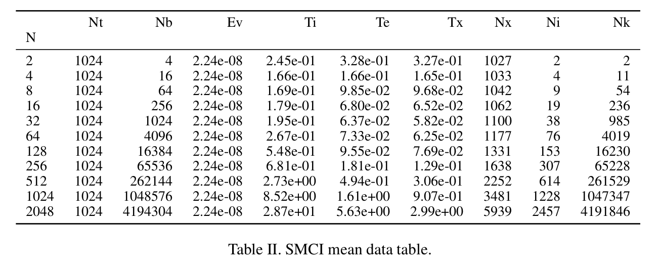
Every time a python script agglomerates data, it can create diagrams and tables and save copies of them in a LaTex directory of your publication / report. In this simple configuration an improvement must be still visually observed in the result, so that a copy of the report is created, then the simulation is executed again with algorithmic modifications, and a new report, filled automatically with data, is compiled from the LaTex source.
A more advanced way of working would be to generate different parameter studies, named after versions of the simulation program, that store data in different sets of files / directories. The python script can then be modified to report all the numbers that were improved. For example: errors that are increased between two executions can be formatted red in the latex output, using a specific formatter, approximately like this:
def red_int_form(x):
	return "\textcolor{red}{%d}" % round(x,1)
Or an overall improvement can be reported: mean, min and max increase and decrease in the error convergence and execution timing.
-
Step 4: Use git hooks to automate test execution on the master branch .
Once steps 1-3 have been set up, automatic execution of the tests can be set up in the simplest sense using git hooks. A release / paper / publication branch can be created that will contain the hooks that call the execution of the test scripts. The test scripts can then create the diagrams and tables as described in steps 1-4 and store them in the report folder (paper/figures, paper/tables), or they can be formatted differently and included into the README.md file on the chosen git branch together with test descriptions. This is a rudimentary solution to automatic testing, compared to using servers such as CDash or Jenkins, but it serves its purpose.
Test automation makes it easy to integrate new code into an existing repository, because adding new tests and extending git hooks will create new data, and additionally, existing tests will be run and evaluated, to make sure that the new implementation does not break any existing code.